2. School of Mechanical Engineering, Nanjing University of Science and Technology, Nanjing 210094, P. R. China
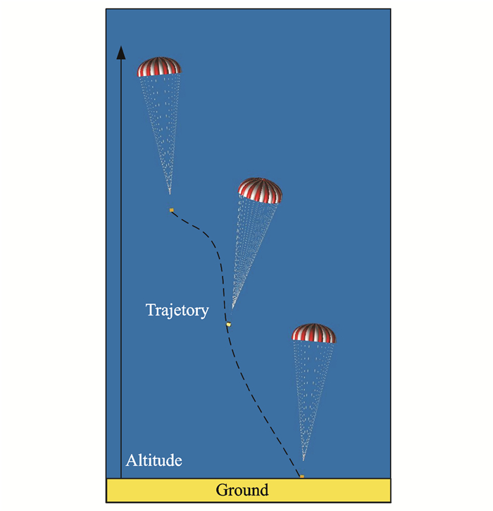
Round parachutes deceleration systems are used in various applications, including airdrop from aircraft, planet entry missions[1, 2]. These applications require the deceleration of pa yload. Most prevailing round parachute decelerator systems are comprised of a sequence of drogue and main parachute (or cluster of parachutes)[3].And during the terminal phase, namely steady descent phase, the systems complete their missions from low speed to the final touch down or splash down speed by mea ns of a passive aerodynamic deceleration, as depicted in Fig. 1. As this phase is the longest, the parachute will experience a fairly long distance which can result in a significant statistical landing deviation.
|
Fig. 1 Trajectory of parachute |
Before ″the Curiosity″ landed successfully, the other rovers dispersed within 100 km[5]. Therefore, great interests in improving landing accuracy [4, 5] have been emerged. Theoretical and experimental studies on parachute(s)-payload path trajectory analysis have been un dertaken for a long time. Previous investigations focued on the descent and landing trajectories of parachute-payload systems, which perform a multibody simu lation adopting limited degree of freedoms rigid body parachute and suspended payload model.
As for airdrop or planet entry missions in practise, landing accuracy is conventionally measured by the circular error probablity, defined as the median miss distance. Although reasonable trajectory simulation for ballistic flight decelerator systems can be performed via the foregoing methods, it is only under a few special initial conditions that the solutions can be obtained due to the complicated process. And those special initial conditions, for instance, include initial velocity of steady descent phase, release altitude, initial angle of attack, parachute bag release direction and definitized wind profile. However, considering that a great variety of problems can be met during the airdrop or planet entry missions in practise, the result set are too limited to cover all cases of the parachute system. There is a typical discrepancy between landing accuracy of simulation and results obtained from flight tests. Monte Carlo methods are developed to study most complicated cases of the decelerator system[6]. Monte Carlo methods were applied to multibody analysis of the system formed by an entry vehicle and a parachute[3]. In his study, the effects of different initial and parachute release conditions were evaluat ed. These analyses provided an elegant method to simulate the ballistic flight ca ses through covering almost all the initial conditions of parachute release states.
In this paper, the Monte Carlo method was applied to the airdrop deviation analysis[7, 8]. Unlike the planet entry problem which only depends on the accuracy of the approach navigation during atmospheric entry, the airdrop system is more dependent on critical parameters, including wind profiles, atmospheric density, mass property uncertainties, and thrust variations, etc. Among them, wind profile is one of the main factors for decelerator system dispersion, which must be addressed during de celerator design in order to estimate delivery accuracy of the system. In addition to the global wind effect, it is also desirable to know how uncertain wind gust relate to error probablity[9].
Different from parafoils which are able to conduct autonomous guide and maneuver to achieve high placement accuracy, the land site of passive decelerator system is more dependent on the wind conditions. The biggest source of uncertainty in the inflight mission is the wind field profile, therefore, it is difficult to construct a suitable wind profile. We emphasize on the dispersion characters under randomized wind conditions. Wind profile is constructed with sections of randomize wind gust. The fluctuating component is generated by pseudo random scheme.
1 Governing Equations of Decelerator System 1.1 Governing equations of parachuteIn this study, a typical parachute-payload system is present. As depicted in Fig. 2, the parachute is constrained by suspension lines. The payload is connected by a set of bridles which converge to the end of the riser. The other end of the riser is connected to suspension lines of the parachute.

|
Fig. 2 Configuration of parachute payload decelerator system |
Decelerator system multibody simulations can both provide realistic altitude history predictions of all bodies throughout the flight and address issues such as design of parachute and suspension lines, desirable elastic properties of the lines, and instrument performance during parachute phase.
It is common practice to assume that the assembly of the parachute and its suspension lines can be considered as rigid in the fully inflated configuration. Namely, deformations in the canopy and elasticity of the suspension lines are neglected. Because the parachute is usually made of very flexible material, this assumption may be different from application of the parachute in real life due to the breathing phenomenon. However, this assumption will greatly simplify the model. This reduced model always correctly reproduces the most relevant features of the trajectory of the decelerator system and has been applied to many parachute trajectory models. In parachute body fixed coordinate frame, the governing equations of a six degree rigid body parachute are written as
| $ {\mathit{\boldsymbol{M}}_{\rm{p}}}\left( {{{\mathit{\boldsymbol{\dot v}}}_{\rm{p}}} + {\mathit{\boldsymbol{ \boldsymbol{\varPhi} }}_{\rm{p}}}{\mathit{\boldsymbol{v}}_{\rm{p}}}} \right) = \mathit{\boldsymbol{R}}_{\rm{p}}^{\rm{T}}{\mathit{\boldsymbol{F}}_{{\rm{p}},{\rm{e}}}} $ | (1) |
| $ {\mathit{\boldsymbol{J}}_{\rm{p}}}{{\mathit{\boldsymbol{\dot \omega }}}_{\rm{p}}} + {\mathit{\boldsymbol{ \boldsymbol{\varPhi} }}_{\rm{p}}}{\mathit{\boldsymbol{J}}_{\rm{p}}}{\mathit{\boldsymbol{\omega }}_{\rm{p}}} = \mathit{\boldsymbol{R}}_{\rm{p}}^{\rm{T}}{\mathit{\boldsymbol{M}}_{{\rm{p}},{\rm{e}}}} $ | (2) |
where Mp is the mass matrix of the parachute, Rp the rotating matrix of parachute body, and Φp the skew matrix of the parachute angular velocity. vp and ωp are the translational and angular velocity vector of parachute, respectively. The equations are written in body fixed coordinate frame except Fp, e and Mp, e. Fp, e is the total force acting on the parachute and Mp, e the total moment acting on the parachute. They are obtained in an inertial reference frame for convenience.
In Eqs.(1), (2), mass terms of the parachute are different from those for a conventional rigid body because the inertial terms include the contribution of parachute unsteady resistance effects. The parachute alters the kinetic energy of the surrounding fluid by means of accelerating the surrounding air and the parachute is affected by the resistance of air when it passes through the air. Since the parachute is made of very light and flexible material, this resistance force cannot be neglected when compared with the parachute inertia force. The effect is conventionally taken into account with the added mass, which is related to the shape, size, motion altitude of the parachute and the atmospheric density[9]. It indicates that added mass effects are significant on the unstable dynamic behavior of the parachute[10]. In this paper, effect of the added mass for the rigid axisymmetric parachute in ideal flow is implemented with the mass matrix[11]. The added mass is often decomposed into apparent and enclosed masses which are air mass contained in the parachute[12].In steady descent state, the breathing phenomenon is neglected, and the parachute volume is invariable. The enclosed mass can be determined by the hemisphere volume
| $ {m_{\rm{a}}} = \frac{1}{{12}}{\rm{ \mathsf{ π} }}D_0^3\rho $ | (3) |
The parachute mass tensor is written as
| $ {\mathit{\boldsymbol{M}}_{\rm{p}}} = \left[ {\begin{array}{*{20}{c}} {{m_{\rm{p}}} + {m_{\rm{a}}}}&0&0\\ 0&{{m_{\rm{p}}} + {m_{\rm{a}}}}&0\\ 0&0&{{m_{\rm{p}}}} \end{array}} \right] $ | (4) |
When the decelerator system is descending, the payload also accelerates the surrounding air. Different from parachute with large reference area, whose component of added mass along the symmetry axis has a strong effect on parachute dynamic stability, the added mass effect can be neglected due to its limited size area and relatively large mass. The governing equations of the six degree of freedom rigid payload are written as a conventional form
| $ m\left( {{{\mathit{\boldsymbol{\dot v}}}_{{\rm{pl}}}} + {\mathit{\boldsymbol{ \boldsymbol{\varPhi} }}_{{\rm{pl}}}}{\mathit{\boldsymbol{v}}_{{\rm{pl}}}}} \right) = \mathit{\boldsymbol{R}}_{{\rm{pl}}}^{\rm{T}}{\mathit{\boldsymbol{F}}_{{\rm{pl}},{\rm{e}}}} $ | (5) |
| $ {\mathit{\boldsymbol{J}}_{{\rm{pl}}}}{{\mathit{\boldsymbol{\dot \omega }}}_{{\rm{pl}}}} + {\mathit{\boldsymbol{ \boldsymbol{\varPhi} }}_{{\rm{pl}}}}\mathit{\boldsymbol{J}}{\mathit{\boldsymbol{\omega }}_{{\rm{pl}}}} = \mathit{\boldsymbol{R}}_{{\rm{pl}}}^{\rm{T}}{\mathit{\boldsymbol{M}}_{{\rm{pl}},{\rm{e}}}} $ | (6) |
where vpl and ωpl are the translational and angular velocity vector of the parachute, respectively, and Rpl is the rotating matrix of payload.
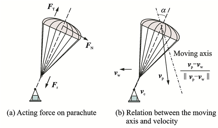
1.3 Acting force on parachuteIt is considered that the assembly of the fully inflated parachute and its suspension lines are rigid body. Therefore, acting force on the parachute is comprised of two parts including the aerodynamic force and the force transmitted via the riser, as depicted in Fig. 3(a).
|
Fig. 3 Sketch of acting force on parachute |
The aerodynamic force consists of steady and unsteady resistance. The unsteady resistance to the parachute in the air is considered as the added mass and implemented in the foregoing analysis.
| $ {\mathit{\boldsymbol{F}}_{\rm{p}}} = {\mathit{\boldsymbol{F}}_{{\rm{pa}}}} + {\mathit{\boldsymbol{F}}_{\rm{r}}} $ | (7) |
where Fpa is the aerodynamic force of the parachute, and Fr the force obtained by the riser.
The steady aerodynamic force of the parachute can be written as
| $ {\mathit{\boldsymbol{F}}_{{\rm{pa}}}} = {C_{{\rm{T}},{\rm{p}}}}\left( {\int_\mathit{\Gamma } {{\mathit{\boldsymbol{p}}_{\rm{p}}}{\rm{d}}{\mathit{\boldsymbol{A}}_{\rm{p}}}} } \right){\mathit{\boldsymbol{e}}_{\rm{T}}} + {C_{{\rm{N}},{\rm{p}}}}\left( {\int_\mathit{\Gamma } {{\mathit{\boldsymbol{p}}_{\rm{p}}}{\rm{d}}{\mathit{\boldsymbol{A}}_{\rm{p}}}} } \right){\mathit{\boldsymbol{e}}_{\rm{N}}} $ | (8) |
where CT, p and CN, p stand for the tangent force coefficients and normal force coefficients[13]. Stability and unstability of the parachute generally depend on normal force coefficients. Both porosity of the membrane material and structure shape of the parachute have a significant influence on these coefficients. The coefficient values are related to the Mach number and the parachute attack angle.
eT and eN are the unit vectors along and normal to the axisymmetric axis of the parachute, respectively. The direction of velocity axis varies with time accordingly.
As depicted in Fig. 3(b), the attack angle is obtained through parachute velocity and wind velocity[14]. The attack angle of the parachute is defined as
| $ \alpha = \arccos \left( {{\mathit{\boldsymbol{e}}_{\rm{r}}} \cdot {\mathit{\boldsymbol{e}}_{\rm{T}}}} \right) $ | (9) |
The unit vector along the velocity axis is written as
| $ {\mathit{\boldsymbol{e}}_{\rm{r}}} = \frac{{{\mathit{\boldsymbol{v}}_{\rm{p}}} + {\mathit{\boldsymbol{v}}_{\rm{w}}}}}{{\left\| {{\mathit{\boldsymbol{v}}_{\rm{p}}} + {\mathit{\boldsymbol{v}}_{\rm{w}}}} \right\|}} $ | (10) |
The normal vector eN is written as
| $ {\mathit{\boldsymbol{e}}_{\rm{N}}} = \left\{ {\begin{array}{*{20}{c}} {\frac{{{\mathit{\boldsymbol{e}}_{\rm{T}}} \times \left( {{\mathit{\boldsymbol{e}}_{\rm{T}}} \times {\mathit{\boldsymbol{e}}_{\rm{r}}}} \right)}}{{\left\| {{\mathit{\boldsymbol{e}}_{\rm{T}}} \times \left( {{\mathit{\boldsymbol{e}}_{\rm{T}}} \times {\mathit{\boldsymbol{e}}_{\rm{r}}}} \right)} \right\|}}}&{\left\| {{\mathit{\boldsymbol{e}}_{\rm{T}}} \times \left( {{\mathit{\boldsymbol{e}}_{\rm{T}}} \times {\mathit{\boldsymbol{e}}_{\rm{r}}}} \right)} \right\| > 0}\\ 0&{\left\| {{\mathit{\boldsymbol{e}}_{\rm{T}}} \times \left( {{\mathit{\boldsymbol{e}}_{\rm{T}}} \times {\mathit{\boldsymbol{e}}_{\rm{r}}}} \right)} \right\| = 0} \end{array}} \right. $ | (11) |
where eT is the unit vector along the parachute axis. Note that
| $ {\mathit{\boldsymbol{e}}_{\rm{T}}} \times {\mathit{\boldsymbol{e}}_{\rm{T}}} = 0 $ | (12) |
The moment can be written as
| $ {\mathit{\boldsymbol{M}}_{\rm{p}}} = {C_{{\rm{N}},{\rm{p}}}}pA{l_{\rm{p}}}\left( {{\mathit{\boldsymbol{e}}_{\rm{N}}} \times {\mathit{\boldsymbol{e}}_{\rm{T}}}} \right) $ | (13) |
It should be stressed that the aerodynamic force can also be divided into forces in x, y, z directions, as depicted in Fig. 4. The aerodynamic force in x or y direction may be the main source that forces the system to glide in space.

|
Fig. 4 Gliding force of parachute |
1.4 Acting force on payload
The acting force on the payload is comprised of three parts including aerodynamic force, gravity force and forces produced by stretched bridles. The force Fpl is given as
| $ {\mathit{\boldsymbol{F}}_{{\rm{pl}}}} = {\mathit{\boldsymbol{F}}_{{\rm{pla}}}} + \mathit{\boldsymbol{G}} + \sum {{\mathit{\boldsymbol{F}}_i}} $ | (14) |
where Fpla is aerodynamic force of the payload, G the gravity force of the payload, and Fi the i-th bridle force.
Similar to Eq.(8), aerodynamic force of the payload is written as
| $ {\mathit{\boldsymbol{F}}_{{\rm{pla}}}} = {C_{{\rm{T}},{\rm{pl}}}}\left( {\int_\mathit{\Gamma } {{\mathit{\boldsymbol{p}}_{{\rm{pl}}}}{\rm{d}}{\mathit{\boldsymbol{A}}_{{\rm{pl}}}}} } \right){\mathit{\boldsymbol{e}}_{\rm{T}}} + {C_{{\rm{N}},{\rm{pl}}}}\left( {\int_\mathit{\Gamma } {{\mathit{\boldsymbol{p}}_{{\rm{pl}}}}{\rm{d}}{\mathit{\boldsymbol{A}}_{{\rm{pl}}}}} } \right){\mathit{\boldsymbol{e}}_{\rm{N}}} $ | (15) |
where CT, pl and CN, pl stand for the tangent force coefficients and normal force coefficients of the payload structure; ppl is the pressure vector, and Apl the face vector.
The gravity force is written as
| $ \mathit{\boldsymbol{G}} = {m_{{\rm{pl}}}}\mathit{\boldsymbol{g}} $ | (16) |
where g is the gravity acceleration vector. In this paper, the generic suspension dynamic model is adopted[3]. This model provides a high degree of flexibility in implementation of the dynamics. This model can easily instantiate the riser or bridles combination.
The force of the bridle is written as
| $ {\mathit{\boldsymbol{F}}_i} = {k_i}\left( {{p_{l,i}} - {p_{0,i}}} \right){\mathit{\boldsymbol{e}}_{l,i}} $ | (17) |
| $ {p_{l,i}} = \left\| {{\mathit{\boldsymbol{D}}_{\rm{c}}} - {\mathit{\boldsymbol{D}}_{l,i}}} \right\| $ | (18) |
where Dl, i is the absolute coordinates of the i-th attached point, Dc th e absolute location of the confluence point, and p0, i the unstretched length of the bridle or riser. It is assumed that both the bridles and riser use the line properties which do not support compression, and while in tension, they behave as ideal massless spring with stiffness properties. The elastic module is sectional function. The slack case of bridles can be generally defined as
| $ {k_i} = \left\{ {\begin{array}{*{20}{c}} 0&{{p_{l,i}}}\\ {f\left( {{p_{l,i}}} \right)}&{{p_{l,i}} > {p_{0,i}}} \end{array}} \right. $ | (19) |
The moment of the payload
| $ {\mathit{\boldsymbol{M}}_{pl,i}} = {\mathit{\boldsymbol{F}}_i} \times {\mathit{\boldsymbol{L}}_i} $ | (20) |
where Li is the vector from the confluence point to the attached point.
The riser and bridles share similar line force model. Because no mass is defined in the confluence node, parachute force is dependent on the location of the confluence node. It is necessary to find out the position of the confluence point.
| $ {\mathit{\boldsymbol{F}}_{\rm{t}}}\left( {{\mathit{\boldsymbol{D}}_{\rm{c}}}} \right) = \sum\limits_i^n {{\mathit{\boldsymbol{F}}_i} + {\mathit{\boldsymbol{F}}_{\rm{r}}}} = {\bf{0}} $ | (21) |
According to the foregoing assumption, when the decelerator system is implemented with multibody simulation, it is necessary to obtain the force of bridles as well as the riser. In this case, the confluence node is fixed and the forces are calculated via Eq.(1 7). After one integration time step is over and new position of the attached points is obtained, the new location of the confluence point is updated with Eq.(2 1). Repeat this procedure over and over again until the terminal state is achieved.
2 Discretized Random Wind Profile FormulationSince the precise delivery is sensitive to the wind profile during the descent, the wind effect should be fully considered in the trajectory analysis. However, it is impractical and unnecessary to obtain a precise wind history. In this paper, a large number of random wind gust sequences are generated to study the dispersion of parachutes.
Through Eqs.(10), (11), the trajectory is affected by the wind velocity. According to the foregoing proposed parachute-payload system simulation, when the parameter s and the initial condition of the decelerator system are given, the landing site will be determined by this wind profile. The mapping of the payload position and the wind sequence can be written as
| $ \mathit{\boldsymbol{D}}\left( t \right) = {\mathit{\boldsymbol{D}}_{\rm{w}}}\left( {{\mathit{\boldsymbol{v}}_{\rm{w}}}} \right) $ | (22) |
Assuming that the horizontal wind velocity at each point depends on altitude z, it can be represented as the combination of the mean wind speed and a zero-mean fluctuation. Varied with the altitude, a wind sequence can be written as
| $ {{\mathit{\boldsymbol{\tilde V}}}_{\rm{w}}} = {\mathit{\boldsymbol{V}}_{\rm{m}}}\left( z \right) + \mathit{\boldsymbol{\tilde v}}\left( z \right) $ | (23) |
In Eq.(23),
For the purposes of this discussion, z is assumed to be a randomize vector representing the uncertain different observation types.
Assuming the wind gust varies from one zone to another zone and the wind field is discretized along the altitude evenly, that is
| $ {{\hat z}_i} = {z_0} - j \cdot {d_l} $ | (24) |
then the discretized wind profile is written as
| $ {{\mathit{\boldsymbol{\tilde V}}}_{\rm{w}}} = {\mathit{\boldsymbol{V}}_{\rm{m}}}\left( z \right) + {{\mathit{\boldsymbol{\tilde v}}}_j}\;\;\;\;\;{{\hat z}_j} \le z < {{\hat z}_{j + 1}} $ | (25) |
where dl is the distance that shares one wind velocity, as depicted in Fig. 5. The wind is comprised of two parts: the mean velocity of wind Vm and the fluctuating wind gust

|
Fig. 5 One sample of random wind velocity distribution along the altitude |
It should be noted that unlike traditional Monte Carlo method, in the proposed method one fluctuating scheme is considered as one sample. The wind profile generates with pseudo random generation method. Namely, the white noise scheme series generate with different initial values (also known as seed of random series). With different seeds, the pseudo random schemes are different from each other.
The wind sample set can be written as
| $ \mathit{\boldsymbol{ \boldsymbol{\varLambda} }} = \left[ {\begin{array}{*{20}{c}} {{{\mathit{\boldsymbol{\tilde V}}}_{{\rm{w}},0}}}& \cdots &{{{\mathit{\boldsymbol{\tilde V}}}_{{\rm{w}},i}}}& \cdots &{{{\mathit{\boldsymbol{\tilde V}}}_{{\rm{w}},SN}}} \end{array}} \right] $ | (26) |
where
The result set can be written as
| $ {{\mathit{\boldsymbol{\bar D}}}_{\rm{w}}} = \left[ {\begin{array}{*{20}{c}} {{\mathit{\boldsymbol{D}}_{\rm{w}}}\left( {{{\mathit{\boldsymbol{\tilde V}}}_{{\rm{w}},0}}} \right)}& \cdots &{{\mathit{\boldsymbol{D}}_{\rm{w}}}\left( {{{\mathit{\boldsymbol{\tilde V}}}_{{\rm{w}},i}}} \right)}& \cdots &{{\mathit{\boldsymbol{D}}_{\rm{w}}}\left( {{{\mathit{\boldsymbol{\tilde V}}}_{{\rm{w}},SN}}} \right)} \end{array}} \right] $ | (27) |
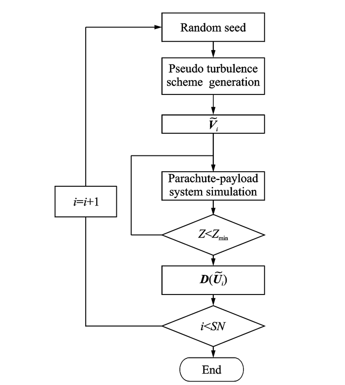
According to the foregoing analysis, when the decelerator system is implemented with the multibody simulation, it is necessary to obtain the wind profile data. In this case, the wind profile generates with pseudo random generation method with different initial values. After the wind profile generates, dynamic and attitude of the parachute-payload can be obtained by means of the proposed method. The flow chart is present in Fig. 6. With this process the response of the parachute-payload system can be studied by virtue of basic knowledge of the atmosphere wind distribution along altitude.
|
Fig. 6 Flow chart of parachute system prediction process |
3 Results and Discussion 3.1 Validation of the payload suspension system
It is clear that one of the most crucial issues when dealing with multibody models of the system, formed by parachute and parachute connected by suspension lines is the representation of actions exchanged between the two bodies through the suspension system.
In this example, a simplified model is studied to validate the proposed system method. In this simplified model, the payload is studied separately without considering the parachute. One end of the riser is fixed.
A suspension system is made of four bridles that connect the payload to the riser which, in turn, connects the confluence point, as depicted in Fig. 7.

|
Fig. 7 Sketch of riser-bridle system |
Together with the characteristics of the suspension system, parameters of the parachute are listed in Table 1.
| Table 1 Parameters of payload |
The elastic module of the bridle and riser is as follows
| $ {k_i} = \left\{ {\begin{array}{*{20}{c}} 0&{{p_{l,i}} \le {p_{0,i}}}\\ {{{10}^6}\;{\rm{N}}/{\rm{m}}}&{{p_{l,i}} > {p_{0,i}}} \end{array}} \right. $ | (28) |
The initial velocity of the payload is [5 0 0] m/s.
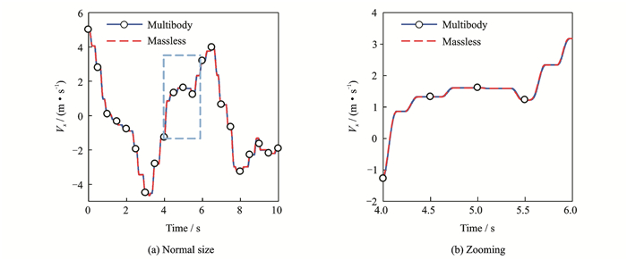
In order to validate the proposed method, we resort to the commercial multibody solver Recurdyn to obtain the reference result. In the Recurdyn solver, the confluence point is modeled as 0.01kg mass point with three translational freedoms. The integration time step is 1×10⁻⁶ s. The proposed method is termed massless method for simplicity. The results are shown in Fig. 8.
|
Fig. 8 Velocity of payload along x direction |
Through these results, it can be concluded that the velocity accords well with the traditional multibody method with very small mass confluence node. The slack of the bridles is manifested clearly in these results.
The difference of the multibody method can be observed in the motion of the confluence point. There is minor difference between time histories of the confluence point position. When the riser falls outside of the nominal solid angle, the tension of the two bridles becomes negative, and the bridles become slack. There will be no force acting on the massless confluence point, as depicted in Fig. 9. Through this example, the suspended system is validated and will be further applied to the following discussion.

|
Fig. 9 Confluence point position along x direction |
3.2 Stability of parachute and its land site distribution
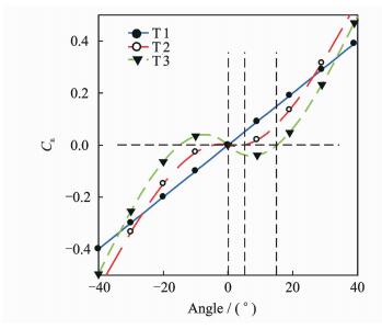
In this example, three types of parachute are discussed and the parameters are shown in Table 2. These parachutes are of same size and same configuration. The main difference is their normal coefficients, which are related to stability of the parachute. It is discovered that the stability of the parachute is mainly determined through porosity of parachute material[13]. When the material of the parachute is less porous, the parachute will be less stable.
| Table 2 Parameters of parachute and payload |
Normal coefficients Cn of three types of parachute are shown in Fig. 10. The angle vs Cn curves are obtained through the CFD method. Static stability is usually evaluated by trim angle of attack[15, 16]. It can be seen that T1 is the most stable parachute yielding relatively small values of trim angle of attack, while T3 is the most unstable parachute and has significantly greater stable attack angles.
|
Fig. 10 Normal coefficients of parachute |
As the randomized scheme is proposed in Section 3, a wide array of information can be produced to estimate the performance of the system. In this example, steady descent parachutes with randomize wind gust model are developed to facilitate the analysis of distribution of the land site.
3.2.1 Two dimensional wind without mean velocityThe velocity of the wind profile is written as
| $ \left\{ \begin{array}{l} {\mathit{\boldsymbol{V}}_{\rm{m}}} = \left[ {\begin{array}{*{20}{c}} 0&0&0 \end{array}} \right]\\ \mathit{\boldsymbol{\tilde v}} = \left[ {\begin{array}{*{20}{c}} {\psi \left( {\varphi - 0.5} \right)}&0&0 \end{array}} \right] \end{array} \right. $ | (29) |
where φ is the uniformly distributed pseudorandom sequence. It is a random vector (mean of zero) that represents the wind gust. ψ is the randomized wind velocity magnitude. In this case, the wind gust is blowing along x direction, so the motion in y direction can be neglected.
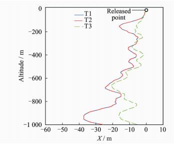
For one sample wind profile, the response of the parachute trajectory along x direction is shown in Fig. 11.
|
Fig. 11 Trajectory of two dimensional wind |
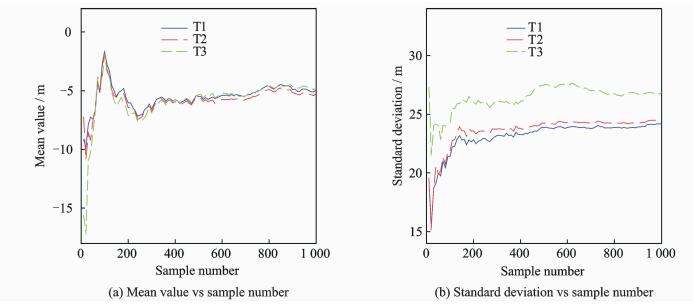
Parachute land site distribution is studied by means of many wind profiles generated through random series with different random seed, as pre-viously mentioned in Section 3. When there is a large quantity of land site results, parameters such as scale σ and mean location μ can be obtained.
Convergence studies of the sample numbers are shown in Fig. 12. The results are expressed by 10—1 000 runs Monte Carlo study. According to the mean value and standard deviation study of the landing site location, it can be seen that the values converge when the sample number is large enough. The distribution of x land site with 1 000 runs is plotted in Fig.13.
|
Fig. 12 Convergence of sample number of normal distributed wind |

|
Fig. 13 Statistical assessment of y location (ψ=8) |
According to the foregoing example, when the parachute is less stable, it tends to have larger trim angle and larger glide force. In this case, the parachute land site tends to have a larger variance.
The land site distribution of the parachute system which experiences different randomized wind gust profiles has been computed. Standard deviation of parachute land site distribution with different randomized wind gust profile is listed in Table 3.
| Table 3 Standard deviation of parachute land site with different randomized wind gust profile |
According to the results, the distribution of the system is dependent on the wind gust magnitude. The dispersion is in proportion to the randomized wind gust velocity with stable parachute, which, however, does not apply to the case when the parachute is not stable.
3.2.2 Three dimensional windThe previous cases are discussed with a two dimensional wind profile. However, the wind profile is always three dimensional. In this case, a full assessment of the dispersion is conducted with a three dimensional wind profile. The velocity of the wind profile is written as
| $ \left\{ \begin{array}{l} {\mathit{\boldsymbol{V}}_{\rm{m}}} = \left[ {\begin{array}{*{20}{c}} 0&0&0 \end{array}} \right]\\ \mathit{\boldsymbol{\tilde v}} = {\left( {\begin{array}{*{20}{c}} {\psi \left( {\phi - 0.5} \right)\cos \left( {2{\rm{ \mathsf{ π} }}\bar \phi } \right)}\\ {\psi \left( {\phi - 0.5} \right)\sin \left( {2{\rm{ \mathsf{ π} }}\bar \phi } \right)}\\ 0 \end{array}} \right)^{\rm{T}}} \end{array} \right. $ | (30) |
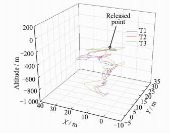
The parachute trajectory with one sample wind profile is depicted in Fig. 14.
|
Fig. 14 3D trajectory of the gravity center of the payload |
In order to study the distribution of the land site location, the scatter plot is used to verify that the generated dispersion falls within the distributions. Through the scatter plot in Fig. 15, the land site has similar distribution to the two dimensional wind profile. And the unstable parachute tends to have larger error probability.

|
Fig. 15 Scatter plot of land sites with 3D wind gusts (ψ=8) |
4 Conclusions
A general parachute-payload model is developed to investigate the descent land site of the decelerator system. This model consists of three parts including the rigid body parachute formulation, the general bridle-riser suspension system formulation, and the randomize win d profile generation formulation. This model has been shown capable of obtaining the distribution of the land site location with different randomized wind profiles.
As the stability of the parachute is usually evaluated by trim angle of attack, three types of parachute with different attack angle normal coefficients are discussed. According to the results, it can be concluded that the landing distribution of the system payload is determined by stability features of a parachute as well as the wind gust profile. In particular, landing site distribution has positive correlation with the velocity magnitude of randomized wind gust profile when the parachute is stable. Because when the parachute deviate from the equilibrium position, it is subject to a steerable force as a restoring force. On the contrast, the landing site distribution has a weak correlation with the randomized wind gust magnitude when the turning point of the normal coefficients is not coincided with the equilibrium point.
Furthermore, it can also be concluded that the mean wind velocity is the major cause which leads to the deviation of the land site and the randomized wind gust is the very one of the factors which leads to the dispersion.
Acknowledgements
This work is supported by the National Natural Science Foundation of China(No.1 1472137);the Educational Commission of Guangdong Province (No.2017KQNCX203), and Science and Technology Project of Guangdong Province (No.2016A010102023, 2017A010102017)
| [1] |
GAO S Y, WANG H T, CHENG W K, et al. Ejection separation characteristic analysis of parachute container cover from return capsule for lunar exploration[J]. Transactions of Nanjing University of Aeronautics and Astronautics, 2014, 31(5): 552-558. |
| [2] |
KLUEVER C A. Entry guidance performance for Mars precision landing[J]. Journal of Guidance, Control, and Dynamics, 2008, 31(6): 1537-1544. DOI:10.2514/1.36950 |
| [3] |
AVANZINI G, GUGLIERI G, TORASSO A. Multibody analysis of terminal phase for a reentry vehicle:A comparative study[J]. Journal of Aircraft, 2012, 49(6): 1940-1952. DOI:10.2514/1.C031788 |
| [4] |
SHEN G, XIA Y, SUN H. A 6DOF mathematical model of parachute in Mars EDL[J]. Advances in Space Research, 2015, 55(7): 1823-1831. DOI:10.1016/j.asr.2015.01.029 |
| [5] |
KORNFELD R P, PRAKASH R, DEVEREAUX A S, et al. Verification and validation of the Mars science laboratory/curiosity rover entry, descent, and landing system[J]. Journal of Spacecraft and Rockets, 2014, 51(4): 1251-1269. DOI:10.2514/1.A32680 |
| [6] |
LAFARGE R A, BATY R S. Functional dependence of trajectory dispersion on initial condition errors[J]. Journal of Spacecraft and Rockets, 1994, 31(5): 806-813. DOI:10.2514/3.26516 |
| [7] |
LIU Cun, TANG Zhili, ZHANG An. Influence of large transport aircraft airdrop conditions on airdrop position error probability[J]. Electronics Optics & Control, 2012, 19(12): 34-37. |
| [8] |
LIU Min, RONG Wei, WANG Weizhi. Monte Carlo method for the parachute-return capsule system[J]. Spacecraft Recovery & Remote Sensing, 2007, 28(1): 18-21. |
| [9] |
CHRISTIAN J A, VERGES A M, BRAUN R D. Statistical reconstruction of mars entry, descent, and landing trajectories and atmospheric profiles: AIAA 2007-6129[R]. USA: AIAA, 2007.
|
| [10] |
EATON J A. Added fluid mass and the equations of motion of a parachute[J]. Aeronautical Quarterly, 2016, 34(3): 226-242. |
| [11] |
GINN J M, CLARK I G, BRAUN R D. Parachute dynamic stability and the effects of apparent inertia[C]//AIAA Atmospheric Flight Mechanics Conference. Atlanta GA: AIAA, 2014: 1-15.
|
| [12] |
FACKRELL S. Study of the added mass of cylinders and spheres[D]. Windsor: University of Windsor, 2011.
|
| [13] |
CRUZ J R, MINECK R E, KELLER D F, et al. Wind tunnel testing of various disk-gap-band parachutes: AIAA Paper 2003-2129[R]. USA: AIAA, 2003.
|
| [14] |
GAO Y H, ZHU F F, ZHANG Y, et al. Wind estimation for UAV based on multi-sensor information fusion[J]. Transactions of Nanjing University of Aeronautics and Astronautics, 2015, 32(1): 42-47. |
| [15] |
Wang Haitao, Qin Zizeng. Dynamic stability simulation in planar motion of parachute system[J]. Journal of System Simulation, 2009, 21(18): 5816-5819. |
| [16] |
COCKRELL D J, HAIDAR N. Influence of the canopy-payload coupling on the dynamic stability in pitch of a parachute system: AIAA Paper 1993-1248[R]. USA: AIAA, 1993.
|
 2018, Vol. 35


